To aggregate is to combine many things into one thing. In databases, there are tools known as aggregate functions or aggregation functions that aggregate a column of data; they combine many rows into one row for a particular column or group of columns. We’ve seen before that a column of data is interchangeable with a list or tuple of values, and that correspondence gives us a good way to give examples of aggregation. If we have a column of grades with values (80.0, 90.0, 95.0, 100.0), there are several ways to aggregate those many values into one value. We can find the largest value in the list (100.0) or the smallest (80.0). We could also add up the values (365.0), count them (4), or compute their average (365.0/4.0 = 91.25). These are all examples of the five aggregation functions we’ll use in I308.
| Aggregate Function |
|---|
| COUNT(column) or COUNT(*) |
| SUM(column) |
| MIN(column) |
| MAX(column) |
| AVG(column) |
Although we only deal with these five in I308 to learn the concept of aggregation, there are many other available ones in a typical DBMS. Aggregation queries are queries that use aggregation functions to roll up a table of data into a single (aggregate) row of data, so it’s a way to simplify information or compute new information that depends on 1 or more rows in a table. All semester long we’ve seen that the FROM and WHERE clause build a table that gets passed to the SELECT clause. Aggregate functions appear in the SELECT clause and condense the information in that table into a single row.
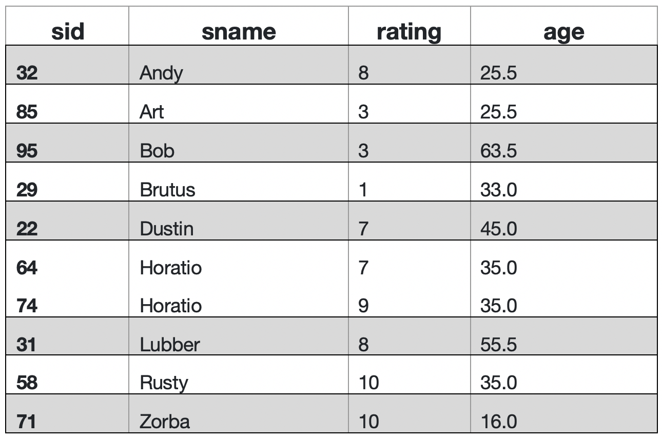
For instance, in the Sailors Reserving Boats database, each sailor has a rating, but together ALL sailors have an average rating. The average rating depends on all the rows in the sailor table, so it’s an aggregate quantity. If we use the Sailors table in the FROM clause but omit the WHERE clause, then the SELECT clause will receive all the rows in the Sailors table. To compute it we write in SQL
SELECT AVG(rating)
FROM Sailors
and see a single number (6.6 as a 1 x 1 table) returned to us with the answer. Note that we passed the name of a single column to the aggregate function AVG. All 5 accept a single column name as their argument. The only one that accepts anything else is COUNT() which also accepts the * wildcard. More on this later.
We can use aggregation with all the SQL bells and whistles we’re used to: “Find the average rating of sailors older than 20 years old.” In this example, since we’ll need a WHERE clause, the SELECT clause does not receive the entire Sailors table. It only receives certain rows. The SELECT clause computes the average of whatever data it receives, so when it receives only some ratings instead of all ratings, we should expect a different average value from the query.
SELECT AVG(rating)
FROM Sailors
WHERE age < 20
Indeed in this case the average rating is returned in a 1×1 table as 10.0, which is greater than the 6.6 average of all sailors’ rating.
One thing to be careful of with aggregation is that you can’t write a query like
SELECT sname, AVG(rating)
FROM Sailors
ever because there are many sname values in the sailors table, but only one average rating. You can’t make a table in SQL that has many rows in the first (sname) column and a single row in the next column. It’s not shaped like a table!
Information Need: “Find the number of sailors.”
SELECT COUNT(*)
FROM Sailors
We just care how many rows are in the table because this table holds records for Sailors. Each row is a sailor. We don’t even need to care about columns. We can thus use * with COUNT instead of the name of any particular column. The interpretation of COUNT(*) is “count rows” without worrying about the values in a particular column. Because we do not have to extract those values and work with them, COUNT(*) can be faster or more efficient, but really it’s just a good practice to use COUNT(*) whenever you know that it’s indeed the rows you’re counting and not particular values.
Information Need: “Find the number of sailors’ names.”
For this one, we need to be a little careful, for we have to worry about the duplicate snames like ‘Horatio’. If we just COUNT(*) we would count Horatio twice, and if we COUNT(sname), we count Horatio twice. We can add the keyword DISTINCT before the column name to remove duplicates:
SELECT COUNT(DISTINCT sname)
FROM Sailors
This one is straightforward
Information Need: “Find the highest rating for any sailor.”
SELECT MAX(rating)
FROM Sailors
But this one below is not. We will have to get the DBMS to compute the highest rating for us as above, but then we have to use that value in the WHERE clause to find which row(s) have ratings with that value.
Information Need: “Find the name of the highest rated sailor.”
SELECT sname
FROM Sailors
WHERE rating = (SELECT MAX(rating)
                              FROM Sailors)
Aggregation queries return a single row, guaranteed. If we have a single column in that single row, it’s a 1×1 table, so we can just use rating = and then put a single-column aggregation query in the () to generate a single value!
Notice I was careful above to say that aggregation returns a single row. We can make multiple-column aggregation queries easily: “Find the average, highest, and lowest ratings for all sailors under 20 years old.”
SELECT AVG(rating) AS avgRating, MAX(rating) as highRating, MIN(rating) AS lowRating
FROM Sailors
WHERE age < 20
The GROUP BY clause
Aggregation queries by design reduce an entire table to one row, and that can be a limitation if one wishes to aggregate over many part of a table at once. Consider the following information need
Information need: For each sailor that has reserved a boat, return their name and the number of reservations they have made.
The result set for this need contains one row per sailor, and each of those contains the result of an aggregation:
| sname | COUNT(*) |
|---|---|
| Dustin | 4 |
| Lubber | 3 |
| Horatio | 2 |
| Horatio | 1 |
To respond to information needs like the previous one, aggregation queries allow an optional clause, GROUP BY, that goes in the same place the ORDER BY clause did (after the WHERE or after FROM if no WHERE clause) and uses the same basic syntax (a comma-separated list of column names). What’s different about GROUP BY is that it splits the table into groups. A group is a set of rows with identical values of the specified column(s), and each group can then be separately aggregated over. Below is the Sailors table GROUPed BY sname. The two sailors of the same nameare in a group together and the other names each lead to groups with only one row each in them.
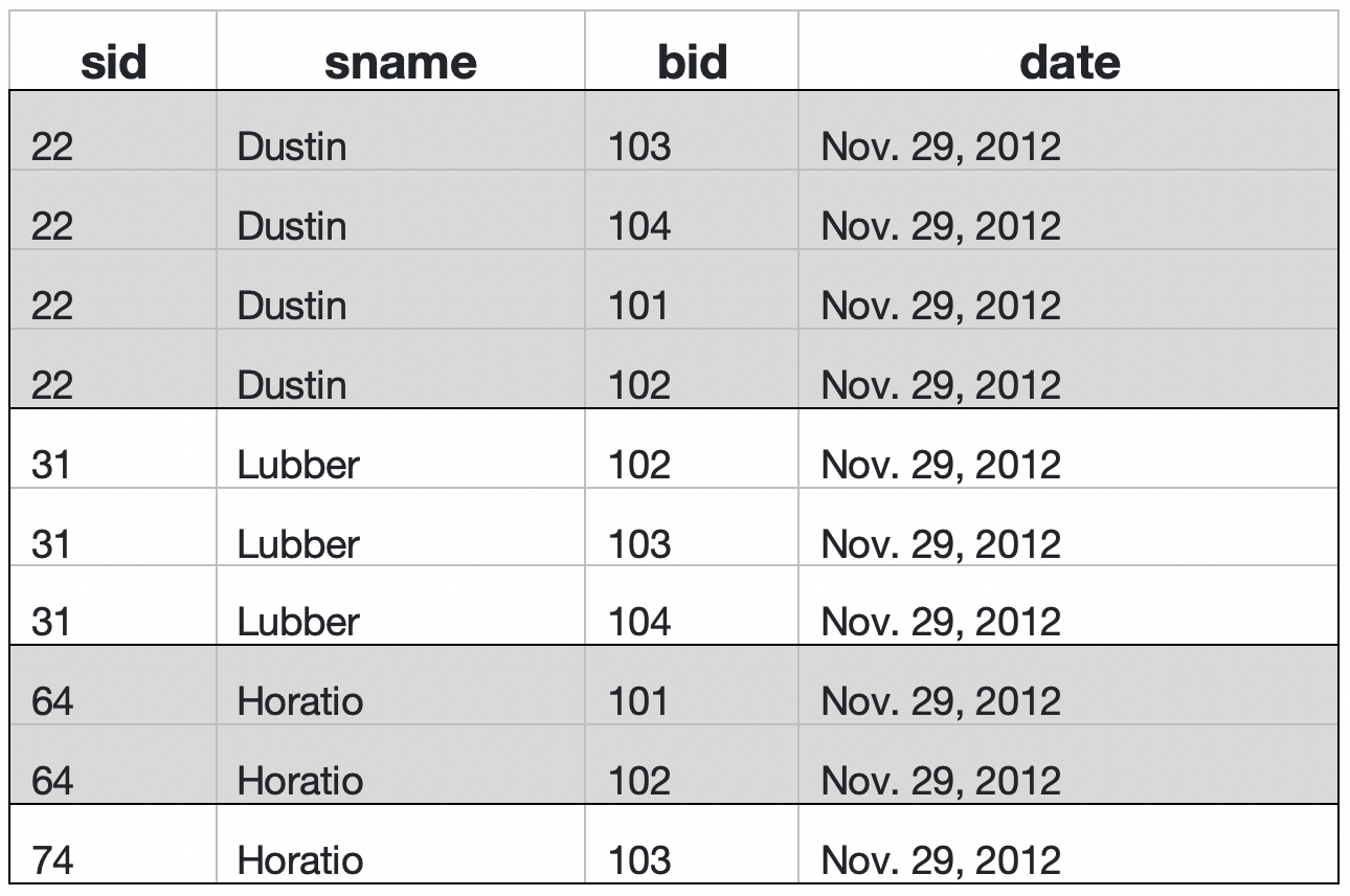
To create a table with groups to answer the information need about the number of reservations for each sailor, we need one group per sailor. Each sailors groups needs to have all that sailors reservations, one row per reservation, in the group. It would like this table:
To generate the query results from the table that is split into groups, we need to return the sname column from each group and the number of rows (COUNT(*)) in each group. With simple aggregation queries (those without groups), we can’t mix single columns and aggregrate functions in our results. When there are groups, we can use columns that have the same value for every row in the group. In the table above, that means we could include sid or sname columns in the result. We leave out side and only include sname because the information need specified only names.
Now that we’ve seen how to visualize the groups and conceptualize the query, let’s write down the SQL. Our strategy will be to JOIN Sailors and Reserves to match up Sailors with their reservations. We’ll then create the groups by adding a GROUP BY clause containing the names of the columns that determine the groups. Since we want one group per sailor, we need to use an sid column since sid is unique for each sailor. Since we want to include sailors’ names in the result, we also need to include the sname column. Finally, we’ll put the sname column and COUNT(*) in the SELECT clause to control the columns in the table we return in response to the information need:
SELECT sname, COUNT(*)
FROM Sailors S INNER JOIN Reserves R ON S.sid = R.sid
GROUP BY sid, sname
That’s the correct way to write this query, so it’s presented first. Many students want to incorrectly write the query as
SELECT sname, COUNT(*)
FROM Sailors S INNER JOIN Reserves R ON S.sid = R.sid
GROUP BY sname
comparing to the correct version, the only difference is that sid is missing in the GROUP BY clause of the incorrect version. Since sname is not a primary key, we will be creating groups of sailors’ names instead of groups of sailors. Sometimes you can get the right answer with this wrong logic. For some instances of a database, there may not be any duplicate names, and then the answer is right. For other instances with duplicate names, we’d get the wrong answer. We have to always write queries to work for any instance of the schema, so we have to use the correct logic.
Whenever we need to group by some record that has a key, we need to use that key to create the groups, even if that key is not returned in the query result
The HAVING clause – A WHERE clause for groups!
Information Need: Find the names of all sailors with a rating above 7 that have 2 or more reservations.
This just got tricky. We can recognize that the rating > 7 is limiting which sailors show up in the results. Since we get to build the table, we can only keep sailors WHERE rating > 7. We haven’t seen a WHERE clause in a GROUP BY query yet, but all the rules we’ve seen this semester still apply. We can put any logic we need in the WHERE clause to filter out rows in the table we’re building before the GROUP BY clause splits that table into groups. If we would like to check that it’s working, we can add the WHERE clause to our previous query
SELECT S.sid, sname, R.bid, R.date
FROM Sailors S INNER JOIN Reserves R ON S.sid = R.sid
WHERE rating > 7
ORDER BY S.sid, sname
If we check the results we’ll see that indeed we have fewer sailors in our result set now:
| sname | COUNT(*) |
|---|---|
| Lubber | 3 |
| Horatio | 1 |
The having 2 or more reservations part of the information need sure sounds like it goes in a where clause, but the problem is we only get the number of reservations by counting rows. And we can only count rows once the groups have been created. The WHERE clause happens before groups are created, so we can’t put COUNT(*) or any other aggregate function in a WHERE clause. We need something like a WHERE clause for aggregation that’s not the WHERE clause. Fortunately there is such a thing; it’s called the HAVING clause. It follows the GROUP BY clause. Like the WHERE clause, it’s optional. If we omit it like we have in the previous queries, then all groups are returned in the answer. If we include it, then we can filter the groups using tests based on aggregate function. We will only receive groups in our final answer that pass the test (evaluate to TRUE).
The WHERE clause test every row, yielding the rows that pass the test. The HAVING clause tests every group, yielding the groups that pass the test.
SELECT sname
FROM Sailors S INNER JOIN Reserves R ON S.sid = R.sid
WHERE rating > 7
GROUP BY sid, sname
HAVING COUNT(*) >= 2
This query returns the following result, indicating that we have indeed filtered groups out of our final result.
| sname | COUNT(*) |
|---|---|
| Lubber | 3 |
In summary, what happens here is that S and R are joined first, and then the rows with a rating > 7 are kept in the result with all other rows discared. So nothing new there. After that, GROUP BY splits the table we’re building into rows with the same sid, sname, i.e. for each sailor. Then HAVING gets its turn and only retains groups containing 2 or more rows. Finally SELECT happens. So long story short: FROM is the first thing the database executes followed by WHERE. Two two create the table to use for the rest of the query. GROUP BY if present splits that table into groups, and HAVING filters the groups. SELECT still happens at the very end of the process to turn the remaining table into a result set responding to the information need.