A warehouse is a place where goods or materials are stored until they are needed. A data warehouse is kind of like that, too. It’s a place where data is stored until it is needed for analysis.
None of the databases we’ve seen this semester are data warehouses. Instead of storing data for later retrieval, they store data for something that is more active, like a company keeping track of employees or a club keeping track of its members. The largest possible examples of databases like these would be ones at places like Amazon or FaceBook where many, many rows are constantly being updated or added to to tables as users purchase items, have their browsing tracked, like friend’s posts, or update their status. These actively-updated databases are called transactional databases, and they tend to be optimized so that data can be quickly added or updated because they change so frequently. The opposite of transactional databases are called analytical databases, and they tend to be optimized for returning large amounts of data in response to queries that allow the end users to carry out more advanced analytics, report generation, or data mining on the data.
Two more technical names for these kinds of databases are OLAP (Online Analytical Processing) and OLTP (Online Transaction Processing). A data warehouse is an example of an OLAP database. Much of its data may come from OLTP databases. For example, Amazon could copy each days sales from its OLTP database every evening to a data warehouse. Analysts at Amazon could then interact with that data without having to burden Amazon’s active transactional database that keeps track of all current activities.
In the same way, many different transactional databases in a company can be warehoused in an OLAP database so that the different data can be combined in order to gain new insights into how effective their business is. This analysis can be used as part of a decision support system to help the business decide on new directions or to gauge the effect of past decisions.
Because OLAP databases serve a different purpose than OLTP ones, they tend to have a different vocabulary which we’ll learn. Even though the vocabulary is different, it’s important to recognize that the databases themselves are pretty much the same. They can still be relational databases made up of tables where each table must have a primary key and foreign keys represent relationships between different rows. The phrase “still be” is used in the previous sentence because not every data warehouse uses the relational model; in I308, though, we’ll only study the ones that do.
OLAP Vocabulary
The most important things that are stored in an OLAP database are called facts. Facts live in tables called fact tables, so a fact is basically a row in a fact table. But it’s more complicated than that, because facts may consist of multiple measures. If we stop and think about this for a second, a fact is a row in a table. We know that rows are made up of a tuple of values with one value per column. So the measures are essentially the values stored in the fact’s row. A fact is a record. A record is a set of related values, and those related values are called measures. As an example, a business might generically keep track of “sales” as their facts. The measures for sales might consist of units sold and prices. Don’t worry about these two definitions too much. Here I’m describing facts as being made of measures, but others treat then as synonyms. A fact tables contains facts or a fact table contains measures; it’s just two different ways of saying the same thing.
Measures get their name because they provide information about the facts that was actually measured (e.g. a number of sales, a rating, a time to complete something, …) Together, the measures make up the fact along with any other information needed to describe what that measurement means. The additional information describing or characterizing measures are dimensions. Since facts may consist of many different measures, facts are multidimensional. In the same way an (x,y,z) point is three-dimensional, a fact with three measures is three-dimensional. A fact with 23 measures would be 23-dimensional, and it would show up as a row in a fact table with at least 23 columns. The example above with two measures is of course, two-dimensionsal.
Continuing with the sales and price example above, we can add dimensions to it as well. Dimensions describe the context of both measures. A business may typically keep track of when and where the sale occurred, so each fact may have a time and location measure associated with it.
The thing that makes OLAP vocabulary and concepts complicated is that dimensions often create a hierarchy for their measure. We’ve seen hierarchical data models before and should recall that a hierarchy is a relationship between items (nodes in the hierarchy) where a node has at most one parent but may have more than one child. The “at most one parent” part reminds us that there is a special node that acts as the root of the hierarchy.
For example, time will be measured in dates, but people using data warehouses to get information often also want weekly summaries, monthly summaries, yearly summaries, etc. We could indicate this hiearchy as day > week > month > year. The most detailed value (day in this example) gives the granularity of the dimension. If the data warehouse records sales for a business and the granularity for time is the day, then the measurements (amount of sales) must be recorded on a daily basis in the warehouse. Not all days must have a measure, but the warehouse must keep track of sales per day. If the company instead tracked sales by the hour, then the granularity would be hour, the data warehouse would need to keep track of any hour in which sales occured, and the hierarchy would become hour > day > week > month > year.
Most often, these hierarchies are drawn out in diagrams to indicate the relationships between the different levels of the hierarchy. The time one described above would look like
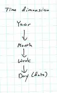
The previous example consisted of the simplest kind of hierarchy where each node had only 1 child. More complicated hierarchies can also arise where there are different ways that could be used to decrease the granularity.
Data Cubes
Here is some sample data for a time & location example of units sold. Every fact will have a pair of values (time,location) that describe it. We can view this data in two different ways. As a plain old database table it would have one fact per row.
| Time | Location | Units SOLD |
|---|---|---|
| 2017 | Indiana | 2 |
| 2017 | Kentucky | 4 |
| 2018 | Indiana | 6 |
| 2018 | Kentucky | 8 |
| 2019 | Indiana | 10 |
| 2019 | Kentucky | 12 |
| 2020 | Indiana | 14 |
| 2020 | Kentucky | 16 |
The more typical way to visualize this data in data warehousing is as a data cube where there are no rows and columns. Instead there are cells with facts, and each cell has a location along each dimension. With two dimensions like time and location, we can think of them as like (x,y) coordinates, and each fact has a set of coordinates associated with it. Because the time and location values are discrete, we can label the x and y axes with the discrete values, and we get a view of the data like the one below.
| Indiana | Kentucky | |
| 2017 | 2 | 4 |
| 2018 | 6 | 8 |
| 2019 | 10 | 12 |
| 2020 | 14 | 16 |
This view of the the data is called a pivot table in the spreadsheet and business analytics worlds. In data warehousing it’s called a two-dimensional data cube or more simply just a data cube. The pivot table concept is pretty much stuck in two dimensions, but the data cube idea generalizes to any number of dimensions. A two dimensional data cube is like a square or spreadsheet, and a three-dimensional one is like an actual cube or a spreadsheet with multiple tabs or sheets. For more than three dimensions it’s more abstract and difficult or impossible to visualized although the terminology is still used.
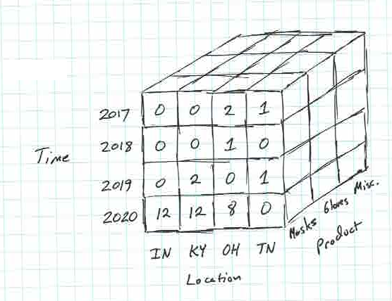
If we add a third dimension product type to the time and location measures, then we can consider a three-dimensional data cube. For any product type, we will be keeping track of time and location measures, so any product type’s sales looks like a two-dimensional data cube.
| Indiana | Kentucky | |
| 2017 | 0 | 0 |
| 2018 | 0 | 0 |
| 2019 | 0 | 2 |
| 2020 | 12 | 12 |
The full data cube for the 3D example looks like, you guessed it, a cube! Here’s a picture illustrating it.
The hierarchies on the dimensions come into play with data cubes. The examples we’ve seen so far didn’t deal with that, so let’s be specific and imagine that time has a granularity of quarters with years at the top level. Location has a granularity of city with state as the top level. The examples we have seen showed top-level (state and year) data, but in general we need to look at lower-level (city and quarter) data, too. It would look like this:
| Jeff Indiana | Clarksville Indiana | Louisville Kentucky | Prospect Kentucky | |
| 2017 Q1 | 1 | |||
| 2017 Q2 | 1 | 2 | ||
| 2017 Q3 | ||||
| 2017 Q4 | 2 | |||
| 2018 Q1 | 1 | 1 | 2 | |
| 2018 Q2 | 2 | 2 | ||
| 2018 Q3 | 2 | 1 | ||
| 2018 Q4 | 1 | 1 | 2 | |
| 2019 Q1 | 1 | 1 | 2 | |
| 2019 Q2 | 1 | 1 | 3 | |
| 2019 Q3 | 1 | 1 | 3 | |
| 2019 Q4 | 4 | 2 | 2 | |
| 2020 Q1 | ||||
| 2020 Q2 | 14 | 4 | 4 | |
| 2020 Q3 | 2 | 3 | ||
| 2020 Q4 | 1 | 2 |
Data Cube Operations
We’ve previously seen that aggregation queries let us look at data in a table in a new way. Instead of viewing all values in a column, we can summarized them in a single column as an average, for instance. Or we can split the data into groups and view statistical summaries by the groups.
Aggregation is the basis for data warehousing analytics, too. The pivot tables showing the top-level (year and state) dimension values above computed those values by aggregating over the lower-level dimension values stored in the fact table. Because data cubes are multidimensional, a bigger vocabulary than just aggregation is used to describe the possible analytics operations. The common data operations data cubes support are are rollups, drilldowns, slicing, and dicing.
| Operation | DefiNition |
|---|---|
| Rollup | Aggregating over one or more dimensions (moving up the hierarchy of a dimension) |
| Drilldown | The inverse of aggregating. Looking at a dimensions in more detail (moving down the hierarchy of a dimension) |
| Slicing | Looking at a particular value of a dimension (taking a slice out of the data cube). |
| Dicing | Looking at ranges of certain dimensions (multiple slices of a data cube) |
Slicing is the likely the easiest of the four operations to deal with. A slice of a data cube means to fix the value of one dimension and look at all the data where the dimension of interest has that fixed value. Two different slices are illustrated below.
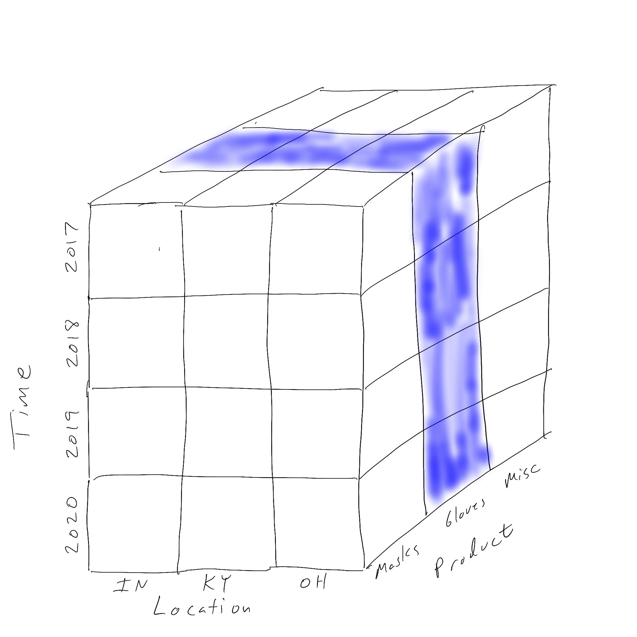
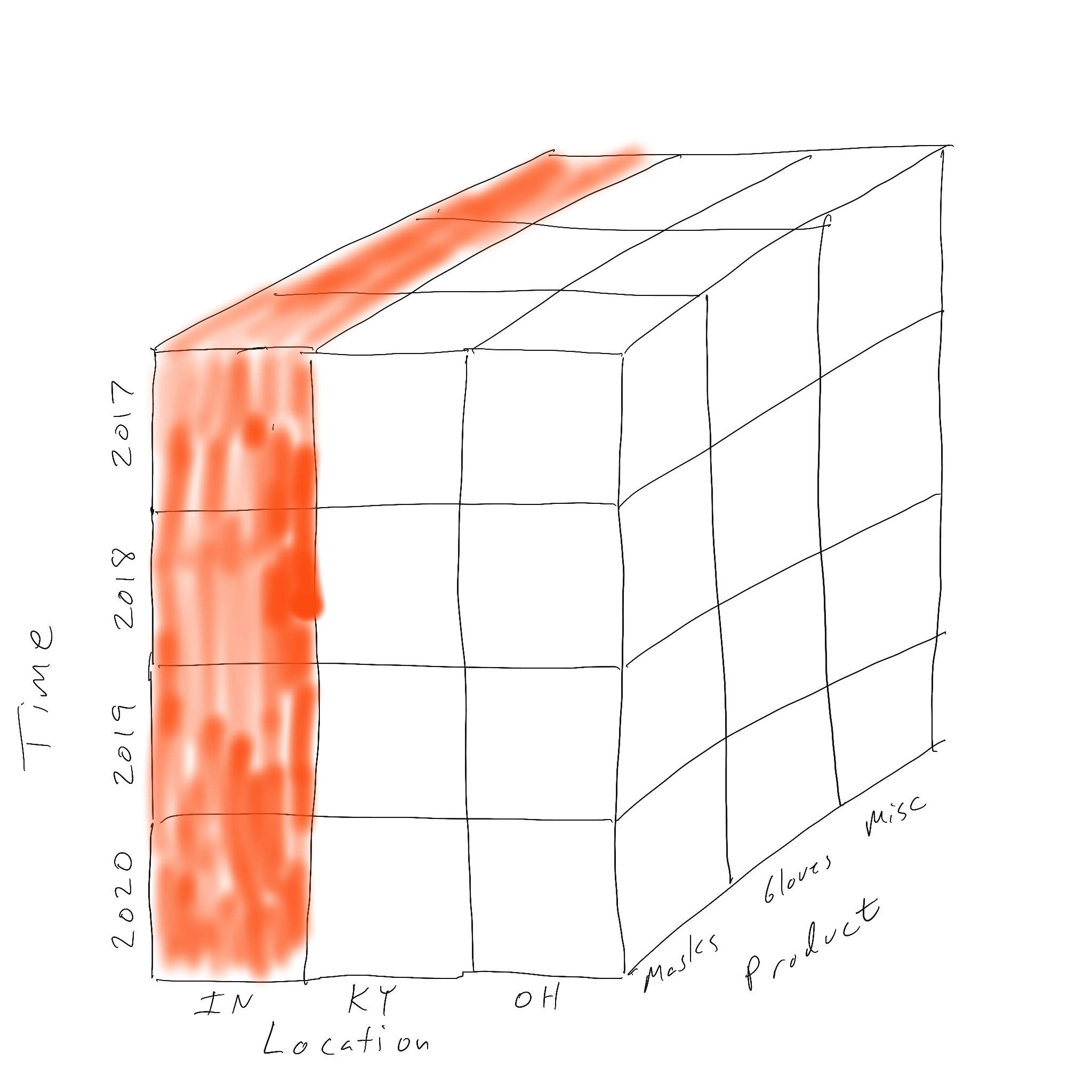
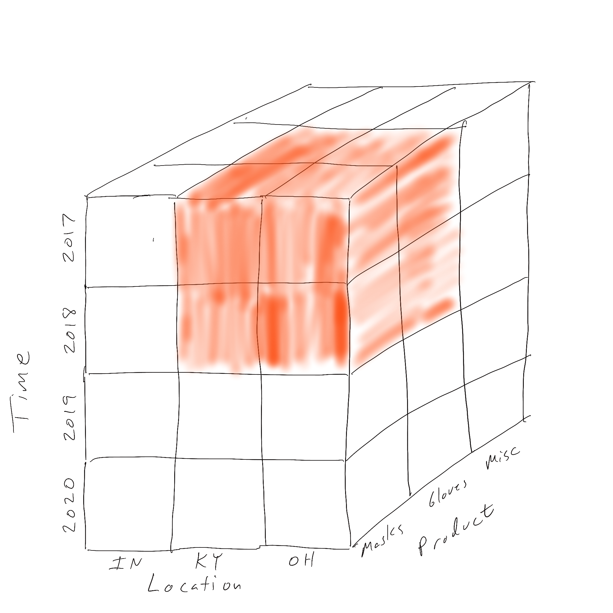
Slicing looks at one fixed value of a dimension. Dicing looks at a range (more than one) of value on two or more dimensions. A dice of our data cube is shown below where all three dimensions’ values have been filtered.
The last two operations, drilldowns and rollups, involve the hierarchies of the dimensions. Slicing and dicing just involve certain values or ranges of a dimensions within the hierarchy, but we never had to worry if we were at the lowest-level (granularity) of the dimension of somewhere above that. Both operations involve changing the data cube along a dimensions, and we can think of the data cube before and after the change.
In a drilldown, we increase the detail along one dimension by moving down the dimension’s hieararchy. A drilldown along the time dimension by starting at year (less detail) and moving down to quarters (more detail) is shown below.
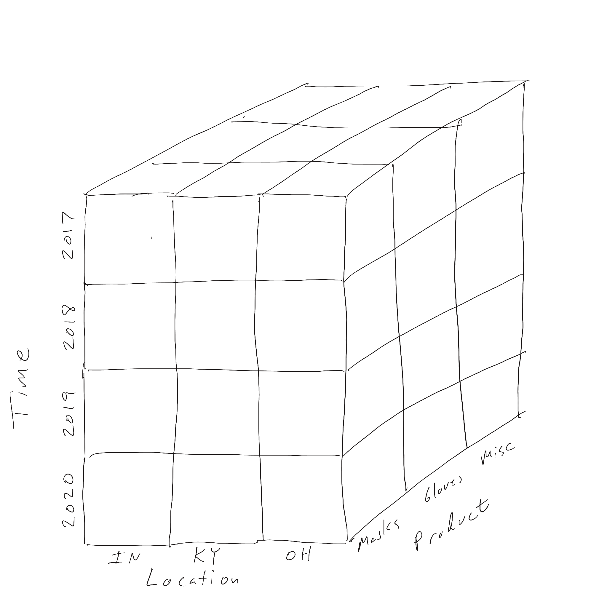
Before Drilldown 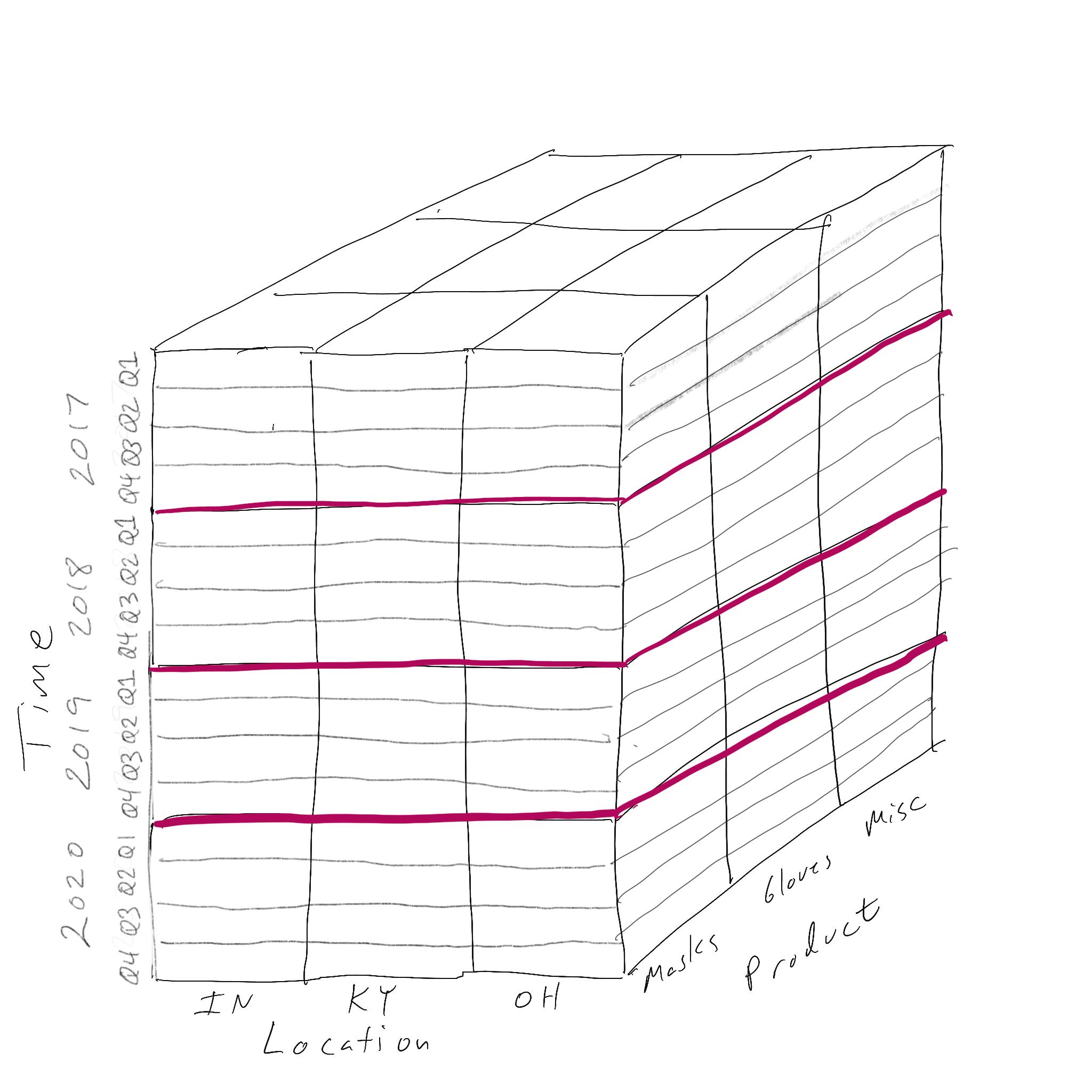
After Drilldown
A rollup is the opposite situation. If we start from a data cube with more detail along a dimension and then move up the hierarchy to view less detail along that dimension, we have “rolled up” that dimension. The nice thing about rolling up is that the terminology is descriptive. One can visualize rolling up (aggregating) each of the four quarters in a year to compute the year’s data.
Before Rollup After Rollup
Star Schemas
Data cubes get emphasized so much in data warehousing because a lot of OLAP databases actually build them, and the OLAP user carrying out data analytics interacts with a data cube to do all their work. They specify what slices or dices to make or what level of the hierarchy to view for a dimension. These kinds of data warehouses are known as MOLAP systems (Multidimensional OLAP). We won’t look at MOLAP systems though, for there is another kind of system, ROLAP (Relational OLAP), that uses relational databases like we’ve seen all semester to store the data. We will focus on ROLAP here, and it’s also worth noting that nowadays MOLAP and data cube concepts are becoming a little bit old-fashioned.
We’ve already seen that the heart of the data warehouse is a fact table, and that every row in the table is a fact. We’ve also seen that the data cube is really just a different way of viewing the data in the fact table. It’s either a re-arrangement of the facts from rows to cells in a cube like we saw with the pivot table, or it may be aggregation over certain dimensions and then a re-arrangement into cells of a cube. In either case, it all starts with a fact table that can be used to associate the facts with their place in the cube based on knowing the values of all the dimensions associated with the facts. So the basic form of a the columns headings in a generic fact table is something like
| Fact 1 | Fact 2 | Fact 3 | Dimension 1 | Dimension 2 | Dimension 3 |
For the example here, we have two facts per row (units sold and price) and three dimensions (Time, Location, and Product Type). We’ve seen that the dimensions typically have a hierarchy, so rather than a single column for a location dimension, we may need multiple columns to describe city, state, region, etc. The time dimensions could also require multiple columns to describe it. So we might end up with a fact table that realistically looked like
| Units Sold | Price | Day | Day of Week | City | State | Region | Product Type |
As soon as we start adding multiple columns per dimension, our fact table is unnormalized. We will have redundancy for all Time columns that have the same Day value. We will have redundancy for all Location columns that represent the same city. We need to normalize the fact table by moving each dimension’s information to a separate table. This decomposition of the facts table gives rise to two kinds of tables in a ROLAP database–fact tables and dimension tables. The fact table contains the measures and each dimension table describes one particular dimension in the data warehouse. Because the decomposition process we’ve learned leads to foreign keys from the original table to the newly-decomposed one, there will be one foreign key from the fact table to each dimension. The schema diagram can be drawn with the fact table in the center surrounded by the dimension tables as shown below.
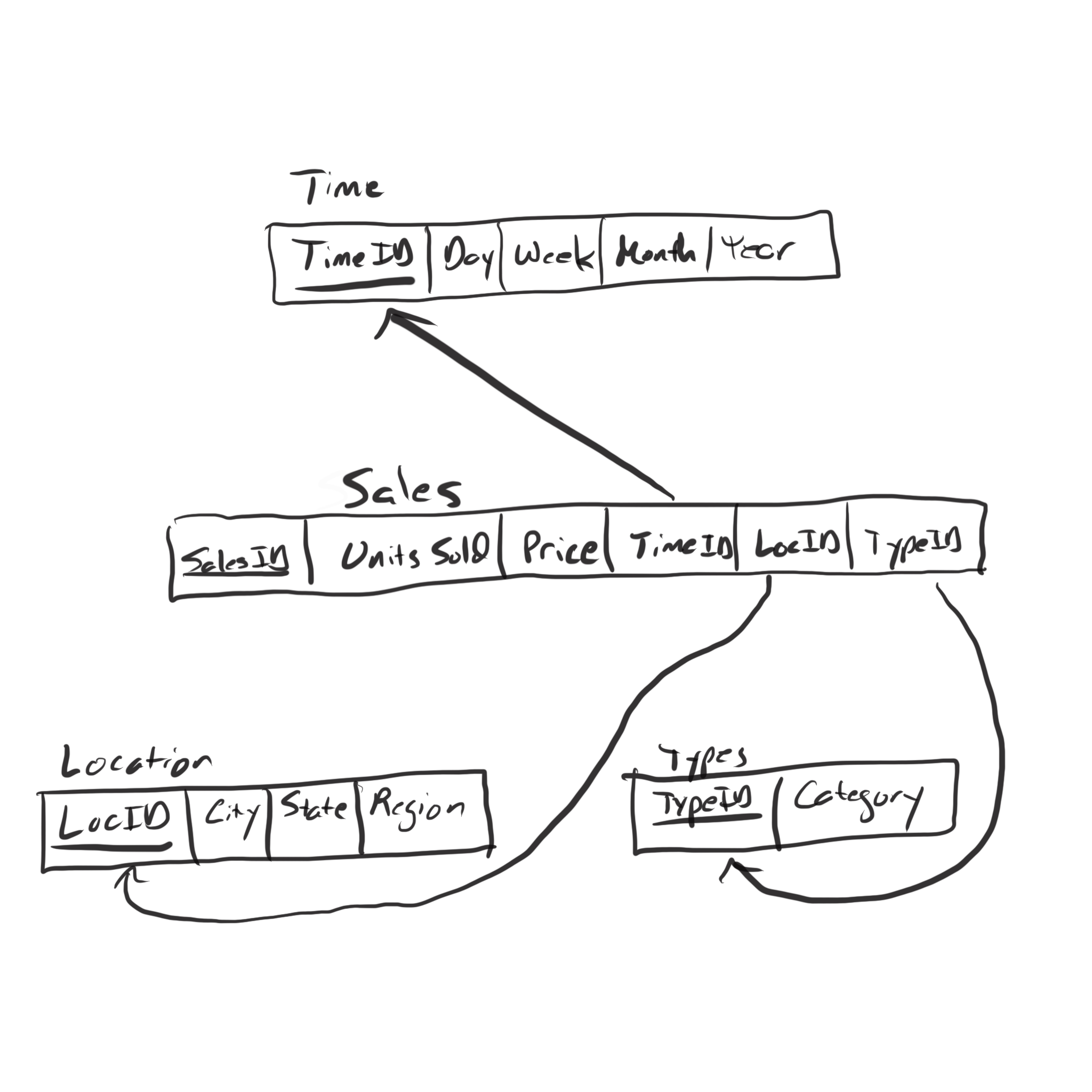
These schemas are called star schemas because the dimension tables “decorate” the fact table like the points of a star decorate its center. We derived the concept by trying to store everything in one table and noting that there would redundancy in the table if we did. In a data warehousing, there are typically very, very many facts, and having redundancy in such a huge table (very, very many rows) leads to unacceptable computational costs. So this normalization is very, very necessary in data warehouses.
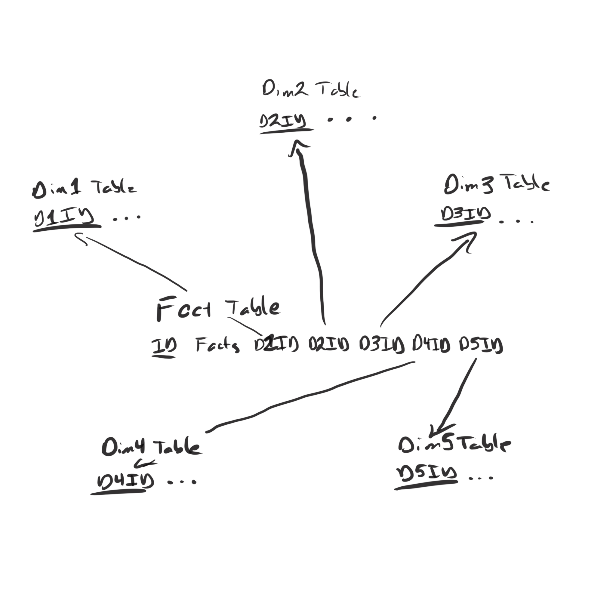
In more detail, in a star schema each dimension gets its own dimension table. it’s common practice to use an id column as the primary key of each dimension table. So we may have a timeid integer primary key instead of using the date as the primary key. The fact table contains one column per measure and one foreign key per dimension. The fact table then has copies of each dimension’s id column, and the arrows point away from the fact table towards the dimension table because the foreign keys in the fact table reference the primary keys in the dimension table.
Since all of these tables are just plain old relational database tables like we’re used to, we would write SELECT FROM WHERE queries on them. Any dimension we use may required joining with that particular dimension table. If we tried to split up the facts into the data cube cells, we would run into trouble and quickly realize the SQL we’ve seen doesn’t quite let us to that. We can add GROUP BY clauses to partition the fact table into groups based on dimensions, but it would be difficult to …
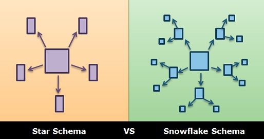
Optional Material: For complicated hierarchies, you could probably convince yourself that some dimensions’ tables would contain redundancy, too. They may also need to be normalized. Normalizing the fact table led to a star; it referenced several tables surrounding it. Normalizing a complicated hierarchy has the same result; there may also be several tables that get referenced by a dimension table. In this kind of schema diagram, the points of the star have little points, too, and it can be drawn resembling a snowflake, and these schemas are in fact called snowflake schemas.