The goal of I427 is for everyone to be able to write their own search engine, assembling each of the components from the previous section into a working program. To do this we will use the Python programming language. Python will be described in detail in the rest of this document. It is used in I427 for a few reasons:
- It has a lightweight syntax. Reading or writing python is very close to reading or writing pseudocode, allowing the programmer to “think” in Python.
- It is well-supported and readily available on most any computing platform
- We can use it effectively through the web browser by working in Jupyter notebooks
- It is well-suited to iteratively and interactively developing working programs from working components (parts of programs)
- For the reasons listed above, Python is a preferred programming language for data scientists and other informaticists
Now that we have understood the basics of IR and the structure of a search engine, we will begin using Python to solve problems or manipulate data in similar ways to the key tasks of search engines. At the start of the course, we will emphasize Python, syntax, and computational thinking over the IR problems we are solving. As the course progresses, we will no longer emphasize that we are learning Python. Instead we will know Python and use it as a tool to solve our problems; we will instead emphasize the IR problems we are solving, the architecture of the search engines we are building, or the design of the programs we are creating.
Students reading these notes should be familiar with Python as a programming language, and they should be able to launch the basic Python interactive interpreter shell and the editor/IDE named Idle in a desktop environment like Windows or OS X. Due to some unfortunate design, standardization, and roadmap decisions made by the powers that be controlling the Python language, there are two common versions of Python in existence—Python 2 and Python 3. The world is gradually (after only a decade) transitioning completely to Python 3, and we use Python 3 in this course. If you run across any Python 2 in this course, that means I missed it in converting the old notes from Python 2 to Python 3. The main Python 2 syntax you may run across is the print statement rather than the Python 3 print() method, but there are also more subtle differences between the two versions of the language that are beyond the scope of I427.
Python is an interpreted language rather than a compiled one. After I110, you should know what this previous sentence means. If you aren’t being taught that in I110, let Kimmer know. For I427 purposes, the fact that Python is interpreted means we can use it interactively. This is one of the big pluses of Python for data science. We can interact with the data and try things out in real time (for small datasets; interacting with larger datasets of course takes longer).
Interacting with Python in I427
Accessing the Linux server for the course
You will receive a login (username) and password for an account on an INFO/CSCI server which runs the Linux operating system. We will interact with this machine primarily through the browser using Jupyter, although you can also connect using ssh software like Putty in Windows, Terminal in MacOS, or the Windows Subsystem for Linux (WSL).
Logging in to Jupyter
Everyone has their own instance of Jupyter running on the server, and each is accessed through an individual URL which will be emailed to you and can be found on Canvas. Upon accessing your URL the first time, you will see a password prompt as shown in Fig. 1. After entering the password correctly, one will see a main screen (Fig. 2) with a list of your files and folders.
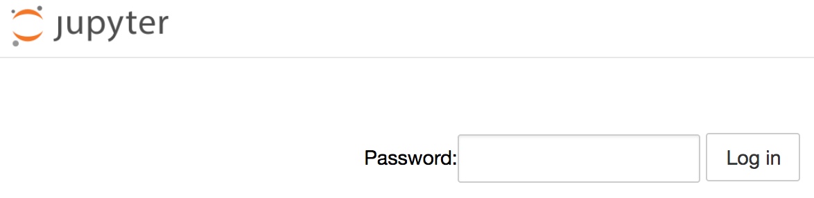
Figure 1: The Jupyter login prompt.
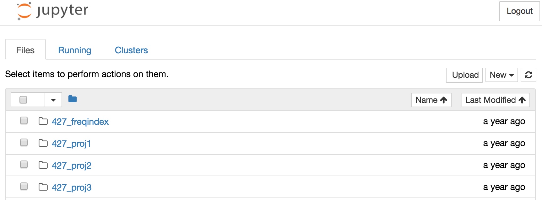
Figure 2: The Jupyter home screen showing folders, notebooks, and basic file management controls.
After logging in to Juptyer with your username and password, you have the option to open either a Jupyter notebook or a shell. First we will interact with the shell to introduce Python, but after today, virtually all your interaction with Jupyter will be by programming in the notebooks. To open the shell from Jupyter, use New > Terminal.
The Linux Shell
The shell presents a command line interface to the user. The default shell is the Bourne-again shell (bash), but other shells are available. Unless you’ve changed your shell, you are running bash. A shell is an interpreter. It waits for user input (terminated by Enter/Return), parses that input, and executes the results. Bash presents the user with a prompt to indicate it is waiting to interpret input. The default prompt resembles
[cjkimmer@ada ~]$
indicating the login name (mine is cjkimmer) and the current working directory (the tilde ~ is a shorthand for a user’s home directory). By default, a user logging in to the system begins in their home directory. All directories have a path from the root of the filesystem (called /), and my home directory’s path is /home/cjkimmer. In addition to being the root, the forward slash (in contrast to stupid Windows backslashes) acts as a level separator. The home directory is a subdirectory of the root, and cjkimmer is a subdirectory of the home directory. The cd command allows you to change your current working directory by specifying absolute paths relative to the root of the hierarchical filesystem (absolute paths start with /) or by specifying relative paths relative to the current working directory. Relative paths do not begin with /. For more information about cd and shell commands in Linux in general, see this tutorial or this one.
From the bash prompt, we will launch the Python interpreter. To do this simply type python and you will be presented with a response similar to what you see below.
[cjkimmer@ada ~]$ python
Python 3.6.3 |Anaconda custom (64-bit)| (default, Oct 13 2017, 12:02:49)
[GCC 7.2.0] on linux
Type "help", "copyright", "credits" or "license" for more information.
>>>
Like bash, the Python interpreter when running interactively prompts the user for input (>>> is the Python prompt), evaluates or parses the result, and returns any output to the user. This process repeats indefinitely until the user exits by calling the quit() method.
[cjkimmer@ada ~]$ python
Python 3.6.3 |Anaconda custom (64-bit)| (default, Oct 13 2017, 12:02:49)
[GCC 7.2.0] on linux
Type "help", "copyright", "credits" or "license" for more information.
>>> x = 2
>>> print(x + 3)
5
>>> quit() [cjkimmer@ada ~]$
This interactive use of an interpreter, either at bash or python prompts, illustrates a Read-eval-print-loop (REPL), so we can speak of using the Python REPL (pronounced “repple”) to accomplish printing the value 5 above. Note that not every python statement causes output to be printed. The print() method does, but the assignment x = 2 does not.
Many servers have multiple installs of Python, and ours is no exception. To find out exactly which python program is invoked by the command, one may execute which python in bash
[cjkimmer@ada ~]$ which python
/usr/local/anaconda3/bin/python
In contrast, the whereis command will display other possible Python installations on the system:
[cjkimmer@ada ~]$ whereis python
python: /usr/bin/python /usr/bin/python2.6 /usr/bin/python2.6-config /usr/lib/python2.6 /usr/lib64/python2.6 /usr/local/bin/python /usr/local/bin /python2.7 /usr/local/bin/python3.3m /usr/local/bin/python3.3 /usr/ local/bin/python3.3m-config /usr/local/bin/python2.7-config /usr/local/ lib/python2.7 /usr/local/lib/python3.3 /usr/local/lib/python2.6 /usr/ include/python2.6 /usr/share/man/man1/python.1.gz
Specifically, whereisand which both search the user’s PATH which is an environment variable containing a list of directories to search for executables corresponding to an issued shell command. Our server runs Red Hat Enterpise Linux (RHEL) which is a very conservative Linux distribution. The system default Python is the Python 2.6 seen in /usr/bin which is not usable for I427. We’ll talk about the difference between Python 2 (old) and Python 3 (new) in class.
The tasks you will most often use the Python interpreter directly for are for testing short code snippets interactively or running a Python file that’s already been saved. (A Python file is simply a text file that contains Python code. Its typical extension is .py.) The previous examples illustrated launching the interpreter for interactive usage. When a Python file is to be interpreted instead, the python command is given the filename as a command-line argument as shown below. We first illustrate the cat (short for catalog) command to view the text file’s contents. For this example, I have created a file print_x.py on the server; you can copy it to to your home directory using the command cp ~cjkimmer/print_x.py . (be sure to include the dot since the second argument of cp is required–here you’re copying it to “dot”) if you’d like to try this example. (The general usage of the cp command is cp source destination, so here the destination is . “dot” which is a shorthand for the current working directory.)
[cjkimmer@ada ~]$ cat print_x.py x=4
print(x)
[cjkimmer@ada ~]$ python print_x.py 4
All that happened here is that the Python interpreter interpreted the file line by line as if we were typing its contents in to the REPL as in the previous example. Before doing that, the file is checked for syntax errors. For instance, if we had messed up and left out the equals sign, we would instead see:
[cjkimmer@ada ~]$ cat print_x.py x4
print(x)
[cjkimmer@ada ~]$ python print_x.py
File "print_x.py", line 1
 x  4
    ^
SyntaxError: invalid syntax
But after the syntax is validated, the file is interpreted. A final useful way to deal with a Python file from the command line is to enter the interactive interpreter after the file has been executed by providing the -i flag :
[cjkimmer@ada ~]$ cat print_x.py
x=4
print(x)
[cjkimmer@ada ~]$ python -i print_x.py 4
>>> y = 6
>>> print(x + y)
10
>>>
Here we see that after the value of x is printed, we get a Python interpreter prompt where we can enter new statements. We also see that we have access to the object x and indeed any other data or functions defined in the Python file that was executed.
This section has illustrated the main ways we may need to use Python from the Linux command line. In the next sections, we will switch to using a Jupyter notebook as our development environment and then focus on the details of the Python language itself.
Jupyter Notebooks
If we have a Python program stored in a .py file, then we may use it from the command line as described above. But we need a way to create our programs as .py files. Because developing a complex program requires debugging, re-designs, or iterative refinement, we need a better environment than the command line interface to do the bulk of our programming work in. I110 should have introduced everyone to at least one option—the IDLE Python IDE (Integrated Development environment). IDLE is straightforward to use and being self-explanatory will not be covered in too much detail here. It contains two primary modes. One is equivalent to the Python interpreter contained in its own graphical window, and the other is a text editor for creating Python source files. These files can then be run inside the interpreter window. Some people like this. By default, IDLE will open with a Python interpreter window (the >>> prompt is a giveaway), but you can change your preferences to open a Python editor window instead. From the command line, you can add a .py file to launch that file in IDLE, e.g. idle listPower.py. When an editor window is open with a file, you can run that file via either the Run menu or the F5 keyboard shortcut. Running is analogous to compiling and then executing a program, but since Python is interpreted, it really launches a new interpreter process that interprets the file line-by-line before then giving you a Python prompt. So, it’s analogous to using python -i with the .py file.
Here we will introduce a better approach for I427—Jupyter notebooks. The customary extension for a Jupyter notebook is .ipynb ( short for Ipython notebook; the Jupyter notebook project was originally called ipython notebooks.). Any files you see ending in .ipynb in your Jupyter home screen can be opened for interactive programming. To create a new one, use New > Python 3 for I427 and note that it’s possible to use other languages like R in Jupyter as well.
Developing in a Jupyter notebook is in many ways similar to interacting with Python REPL directly. Python statements may be entered and evaluated with the output viewed just as with the command-line REPL. The key difference with a Jupyter notebook is that the Python code is entered in cells. A cell is a block of code that is evaluated all at once. Fig. 3 illustrates a basic Jupyter notebook with one cell. The blue highlighted rectangle indicates that it is the active cell. Clicking the ”Play button” or typing Shift + Enter/Return will evaluate the cell. The cell is evaluated line-by-line as if we typed each line one-by-one into the Python interpreter REPL. The advantage of a cell is that we can enter many lines at once, get them right, and then evaluate them as a group. Also, after evaluating the cell, if we find a bug or logic error, we can edit that cell and re-evaluate it. If we enter Python code into many cells and evaluate them all in order, it is equivalent to entering all the code in a REPL. However, if we evaluate cells, edit them and re-evaluate the flow of code becomes a little more abstract. Getting used to programming in notebooks is a key task early in I427.
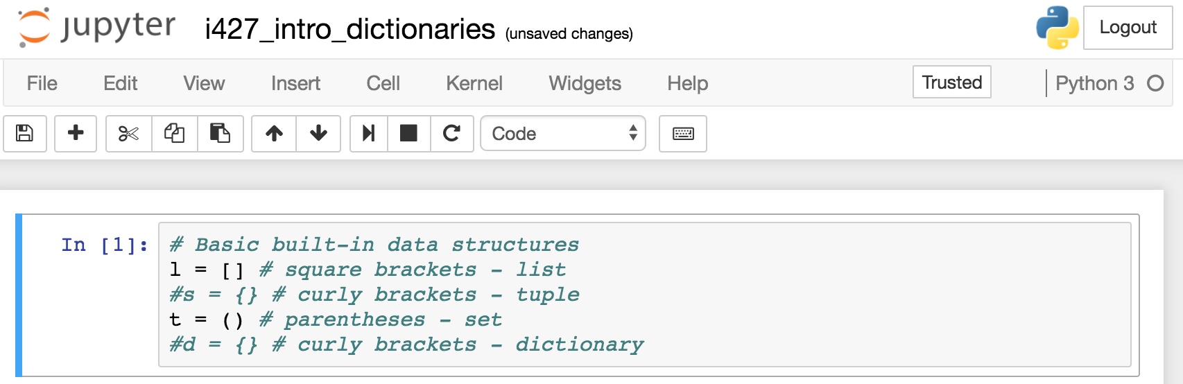
Figure 3: A typical Jupyter notebook showing the GUI widgets and a cell of Python code.
The advantages of using notebooks are many:
- We can iteratively refine or fix our code by editing and re-evaluating cells
- Once we’re happy with our code, we can download the notebook as a .py file
- Juptyer notebooks are highly readable. They don’t just have to have Python code; they may also contain markdown text formatted to make them highly readable and shareable.
- We can access them anywhere we have an Internet connection through a web browser. Once we have working code in a Jupyter notebook, we can use the File menu, select Download As… and then selection Python file (.py) to get a Python version of our Jupyter notebook. Since we downloaded that .py file, it will be on our local machine. To use it on ada as described above with the Python interpreter, we must transfer the file to ada. On a Windows machine, WinSCP is the recommended way to transfer a file. We saw how to do this in I308. Now that we have covered the basics of how we’ll use Python programs in I427, let’s start looking at the language itself to learn what kind of programming we’ll be doing in I427.
I have a video and slides about Jupyter on Canvas that I suggest you watch at this point. If you prefer to stay away from Canvas, then see this tutorial below that starts in the middle of the action since I’ve skipped some unnecessary part about installing Jupyter using Anaconda (a Python distribution) on Windows.
Python variables and objects
Every variable or object in Python has a type associated with it. The fact that everything does have a type known to the Python interpreter means that Python is strongly typed . There are weakly-typed programming languages, but Python is not one of them. Python provides a type function which can be used to inspect the type of an object. When you’re learning someone else’s code or debugging your own, it can be useful to find out the type of an object in this way when you’re not sure, but in a program you write for I427, it’s not likely it will need to have the type() function in it.
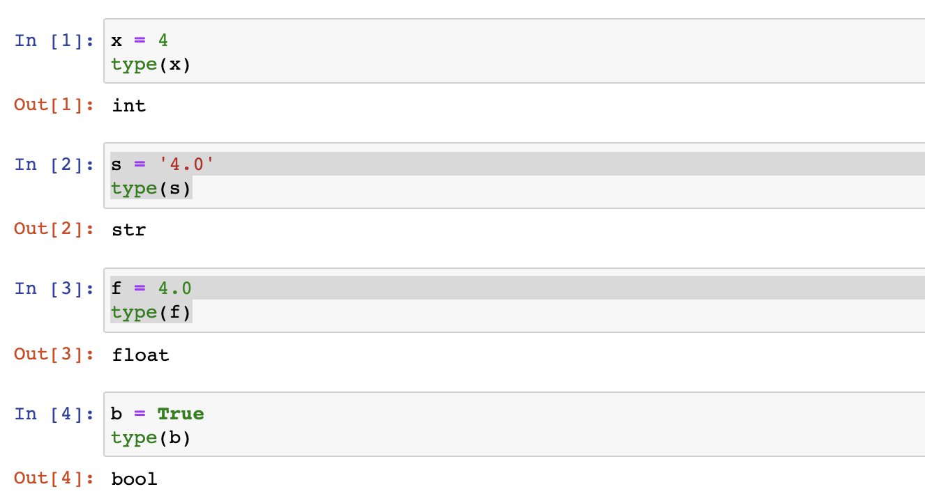
The above code snippet illustrates a few things beyond the type() function. It illustrates the two primitive numeric types int and float along with some other primitive types str and bool. We can also see that not only is int a type, it is a class, and we can more properly refer to x as an object rather than a variable. In other words, as an object of type int, x is an instance of the class int. int is a built-in type in Python, but we can also define our own classes if we need to. The fact that these types have a class associated with them indicating that Python is object-oriented. Note that the value True begins with a capital letter while bool begins with lowercase. Built-in types in Python begin with lowercase letters. A final thing to note is that its irrelevant that we used the print() function or just evaluated the type() method directly. When our statement contains a return value that is not assigned to an object, the result of that value is output by the interpreter.
In addition to being strongly typed, Python is also dynamically typed. Dynamic typing means that a symbol can have objects of multiple different types associated with it during the life of a program. In Python, the object x may change type; this is not a feat that one could achieve in a statically-typed language like Java.
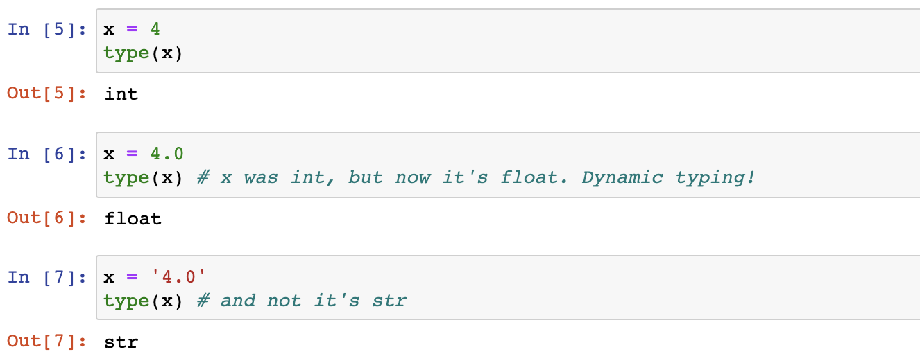
One important concept to keep in mind for variable names in Python is that they are most like references to an object (similar to in Java). So when x is assigned a new value each time above, the reference changes. At first x references or points to an int, but then it references or points to a float instead. Its type changes by pointing to something different; the int 4 does not magically morph into a float 4. In light of this, many developers think of variables in Python as labels or simply names. They provide a name or label for the object the reference; they’re not quite the same as that object.
Just because the type referenced by a variable name can change doesn’t mean that it should. As a rule of thumb in I427, never assign a value of a different type to an existing variable name in your production code. In dev or exploratory code you may find that you re-design or reconsider your approach so that you re-use a name to hold data of a different type. This is part of the Python development process. Once your code is finalized, though, a name should only reference objects of a single type since it’s confusing if you don’t follow this rule. Is x an int at this point in the program, or has it now switched to a str? In general, anything that could potentially confuse the programmer when the programmer tries to think about their code should be avoided.
It is useful to be able to change the type of an object while debugging or developing code. If an object needs to be modified to make the program work, it’s not a problem! Likewise, functions (coming later) are dynamic and can be redefined during a Python program to have the same name and perform different steps or even return different things. But in the final version of the program, all objects and functions should be finalized. Behind the scenes, objects like x hold a reference to a value, and that reference may reference values of any type. Changing the type of an object x in code then simply amounts to the Python runtime changing what x points to (references).
The advantage of a dynamically-typed language is that you don’t have to waste time declaring the type of an object. You can just assign to a name, and the Python interpreter will give that name whatever type of the object it holds. This can greatly speed up development. The disadvantage is that the programmer either needs to remember what type they think a name should hold. Ideally, they can document with comments what type(s) they think should be stored in a particular object.
Semantic Indentation
Python uses semantic indentation which is a way of saying that the level of indentation of a line of code can by syntactically significant in the program. In particular indentation is used to indicate blocks of code with the same scope. In Java, such blocks are indicated by curly brace pairs { and }, and remembering this helps remind you when you need to indent blocks of Python. Bodies of functions, the bodies of if and else, and the bodies of loops are all indented with respect to the line of code that begins the bodies.
Since we’ve already seen the bool type, let’s use an if statement first.
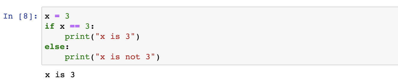
This example is the first time we’ve seen a block of code in Python that forms its own scope—the bodies of the two branches of the if statement. Such blocks in Python are introduced by the : at the end of the line beginning the block. Each successive line in the block is indented with a tab. The Python REPL indicates the indented block with … and the indented code. To terminate a block, merely type Enter/return on a blank line. In this case, terminating the block causes the multiline if statement to execute.
Objects in Python
We’ve already seen that in IR we work with a corpus, a collection of documents. Each document must be tokenized in order to determine which possible search terms it might contain. The most naive way to handle these aspects is to store each document as a string and then use each word in a document as a token. Presumably spaces separate words. The code below puts that plan into action.
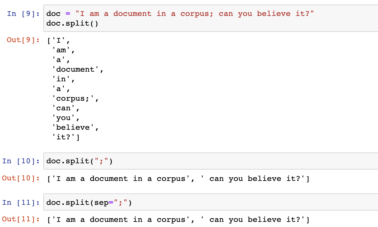
The doc object is of type str. str is the class and doc is an instance of that class. A class is a collection of data and functions that act on that data. Here the data is the value held by the str object, and the methods can be found here or by Googling something like “Python string class reference”. The split() method is used above. Note that the syntax for invoking a function on an object is the same as Java. It’s object_name.method_name() to do so. By default when no argument is supplied in the (), it uses spaces to determine the separate parts of the string, and it returns not one str but a collection of them. A list of them in fact. In Python, a collection of values in [] separated by commas indicates that the values together comprise a single object of type list (list is a class).
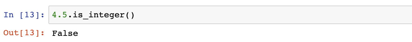
Strings are not the only built-in class the provides methods. The others we have already seen do, too. And in fact, we don’t have to use a variable to invoke the method. We can also use a hard-coded value because at run-time the variable symbol evaluates to its value, if any, anyway.
Returning to Fig. 7, we can also note that the split() method works in several different ways. By default, it splits on whitespace, but we can pass a value to override that behavior. We can also achieve the same result by naming that value we pass in sep. These different behaviors illustrate how Python handles function arguments with default variables. Since the one called sep is the first value, using its name is optional, but we can use its name to explicitly indicate which value we’re overriding. We’ll talk more about these concepts later.