Schema Refinement

After following the process we’ve seen for converting and ERD into a relational database schema, we are guaranteed to have a collection of tables that follow the relational model and capture all the relationships between records. Since all the information in the relationships is reflected in the tables, columns, and foreign keys and key pairings, we can write SELECT FROM WHERE queries using INNER JOINs to retrieve any valid information we need from the database.

Although the resulting schema will be successful from that perspective described above, there are still subtle issues that can arise in the database involving redundancy (duplicated data). Schemas with these issues need to be modified to an equivalent version that doesn’t have the issues. This modification in the initial schema to a final version is called schema refinement or normalization.

The goal of schema refinement is thus to eliminate or minimize the redundancy of tables. Doing so prevents situations the anomalies we saw when first learning about the relational model:

• Insertion anomaly – if data are redundant, you may find it necessary to add copies of existing data in the database when you try to add brand new data.
• Update anomaly – if you need to edit data that exists in many places, you have to make sure to edit it in all places
• Deletion anomaly – if you delete data that exists in many places, you need to delete it everywhere

Schema refinement is a way to prevent as many of these anomalies as possible because schema diagrams created from ERDs cannot be guaranteed to be free of these problems.

Functional Dependencies

In order to guarantee that there will be no issues with redundancy in a database, database designers, informaticists, and computer scientists use a somewhat mathematical notion of a functional dependency. A functional dependency (FD) is a relationship between two groups or sets of columns in a table where the value of one group of columns can be used to predict or determine the value of another group. Sometimes this notion of predicting or determining can means there’s an actual bona fide mathematical function involved. For instance if we had a table named Weights that had Pounds and Newtons columns, we would know that there is a formula relating their values: Newtons = 4.45 Pounds. With this formula, it’s easy to see that the value in the column is what matters and not what row in a table it’s in. Anytime we have a value of 1 Pound in a row, the existence of the functional dependency guarantees that the value in the Newtons column in that row will be 4.45. All 1 Pound rows in the table will also be 4.45 Newton rows.

Functional dependencies don’t have to result from a mathematical formula, though. It’s more common that one column can be used to “look up” the values in other columns. In fact, that’s how we use primary keys in a database. So a primary key column like and employee ID or an SSN in a table of employees can be used to “predict” the employee’s name, address, etc. just because the value is unique to that employee despite the lack of a formula.

We use a notation A → B to write down functional dependencies and we read it as “column A determines column B”. When more than one column is involved on either side of the arrow, we simply write them as a comma-separated list of column names. A,C → B,D means that the two values of columns A and C determine both columns B and D. It’s the same as A,C → B and A,C → D, emphasizing that B and D are in some sense independent while it’s the pair of values in columns A and C that must be taken together and not separately. The value(s) of the column(s) on the left hand side of the arrow determine the value(s) of the column(s) on the right hand side of the arrow. Also note that the columns need to all belong to the same table. Just because the employee table has a functional dependency involving a SSN doesn’t mean that other tables containing that same kind of column have to. The same “for all rows” logic from the Pounds → Newtons example applies for any FD. All rows in a table with identical values in column A will also be rows that have identical values stored in column B. If it involves more than one column like A,C → D, then all columns with a particular pair of (A,C) values will also have the same column D values.

The main goal of schema refinement is to ensure that the only functional dependencies a table has are on a key. A functional dependency “on” a column or columns means it’s on the left hand side of the arrow side, so the main goal when normalizing is to only have FDs like key column(s) → non-key column(s). There’s even a saying for this:

Data should depend on the key, the whole key, and nothing but the key.

We’ll see that this process of normalization involves make sure each table in your database meets constraints specified by so-called “normal forms” that relate to the functional dependencies a table has. When a table has a “bad” functional dependency that breaks a rule of a normal form, the table needs to be decomposed (split) into more than one table to fix the problem. First we see how this decomposition works, and then we discuss the normal forms.

Decomposition to Eliminate Redundancy

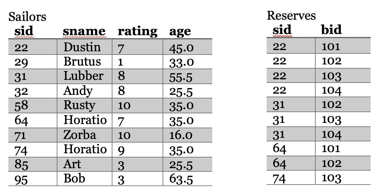
Here’s a table called Reservations that has some redundancy in it:

sid	sname	rating	age	bid	date
22	Dustin	7	45.0	101	Nov. 29, 2012
22	Dustin	7	45.0	102	Nov. 29, 2012
22	Dustin	7	45.0	103	Nov. 29, 2012
22	Dustin	7	45.0	104	Nov. 29, 2012
31	Lubber	8	55.5	102	Nov. 29, 2012
31	Lubber	8	55.5	103	Nov. 29, 2012
31	Lubber	8	55.5	104	Nov. 29, 2012
64	Horatio	7	35.0	101	Nov. 29, 2012

The FD in Reservations is sid → sname, rating, age . We can verify that all rows with the same sid value (all 4 sid = 22 rows, for instance) also have matching sname, rating, and age values. Because sid is not the primary key (it can’t be because many rows have the same sid value), that means the group of columns (sid, sname, rating, age) are redundant in the table. Maintaining the Reservations table would be a headache because anomalies in the data could arise if one is not careful.

The solution is to decompose Reservations to eliminate the redundancy. A decomposition to eliminate redundancy is a splitting of one table into two or more tables that can be joined back together to recover all the initial information. Such a decomposition is called a lossless decomposition because INNER JOINs can be used to regenerate or recover all the initial information.

When we have an FD that generates redundancy like the sid → sname, rating, age one above, we carry out a decomposition by making a new table that contains all the columns in this “bad FD”. This new table won’t in general contain as many rows as the original table because we remove duplicate rows. So the new table with sid, sname, rating, and age columns will be

sid	sname	rating	age
22	Dustin	7	45.0
31	Lubber	8	55.5
64	Horatio	7	35.0

This new table still has the sid → sname, rating, age FD in it. By removing duplicate rows, though, we can have a table where sid is the primary key. When the columns(s) on the left hand side of the arrow in an FD are the primary key, then redundancy is eliminated because any value of the primary key will appear at most one time in the table. So PK column → other columns is a “good” FD that won’t have redundancy issues. In the original Reservations table, that dependency was not on the primary key (sid wasn’t the PK, remember). Dependencies that are not on the primary key are usually bad ones that will create redundancies. By moving that FD to a new table, we have preserved the FD (it still exists with sid determining the other columns’ values) but converted it from a bad one to a good one.

To finish the decomposition of Reservations to eliminate redundancy, we need to remove the columns on the right hand side of the → from the Reservations table. We keep the one on the left hand side of the → in the original table, still. So in this example, sid stays in Reservations and sname, age, and rating are removed. Their removal is OK since they’re now safe and sound in the new Sailors table we made. The original becomes

sid	bid	date
22	101	Nov. 29, 2012
22	102	Nov. 29, 2012
22	103	Nov. 29, 2012
22	104	Nov. 29, 2012
31	102	Nov. 29, 2012
31	103	Nov. 29, 2012
31	104	Nov. 29, 2012
64	101	Nov. 29, 2012

The reason we keep the sid column but not the other is that the sid column makes the decomposition lossless. We can use INNER JOIN on the two tables and match up corresponding rows based on having the same sid value. When we carry out that INNER JOIN, we recover the original table! For this to work, that means sid needs to be a foreign key in the original table referencing the sid primary key of the new table. This idea is made more clear in before and after schema diagrams showing the decomposition to eliminate redundancy.

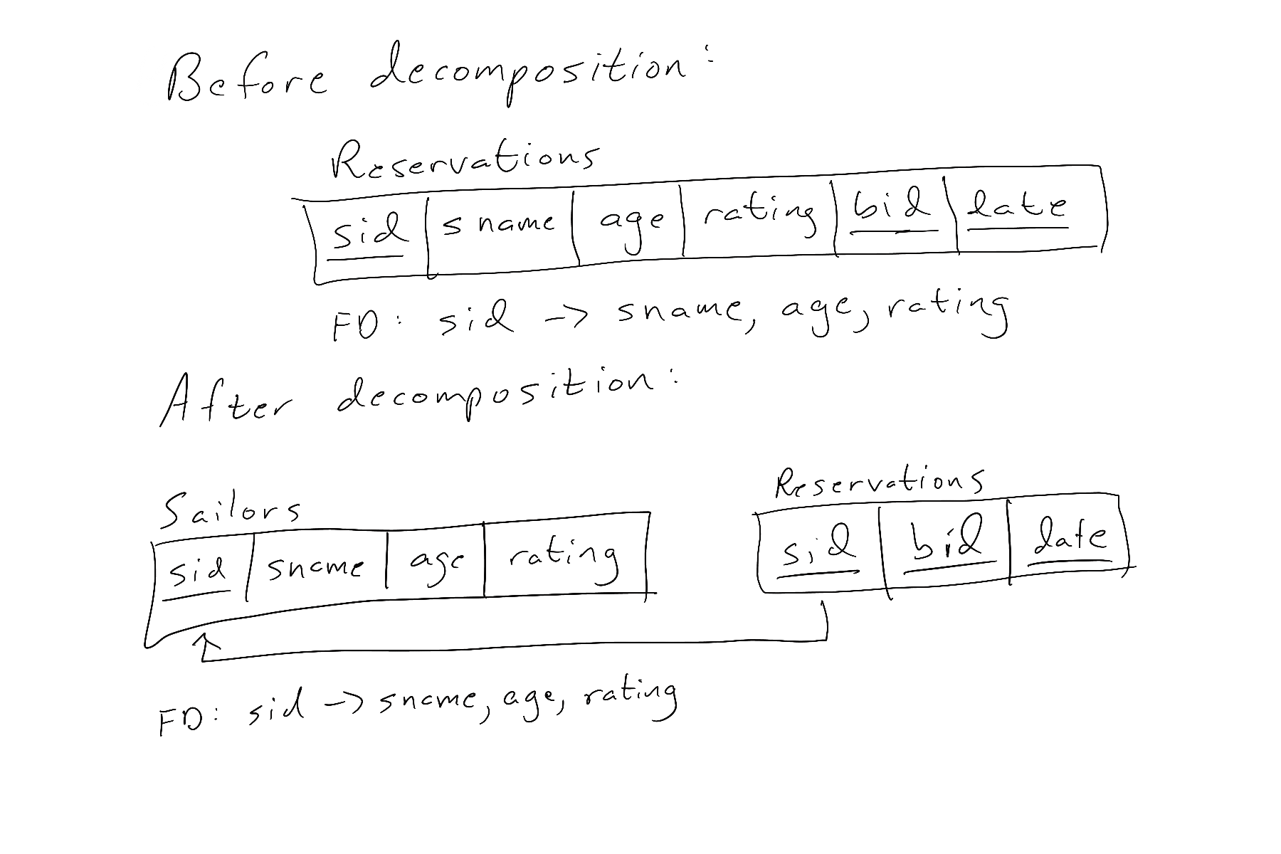
In summary, decomposition to eliminate redundancy is a three-step process. When we have a “bad” FD causing redundancy in a table, we need to carry out a lossless decomposition on that table to eliminate the redundancy. The steps are:

1. Create a new table containing all the columns in the bad FD. The columns on the left-hand side of the FD will be the primary key of the new table. Remove any duplicate rows in the table so that every row is unique.
2. Remove the columns on the right hand side of the FD from the original table.
3. Make the columns on the left hand side of the FD foreign keys in the original table.

If we have a table with redundancy and only one “bad” FD, then we end up with two tables instead of one after decomposition. It’s possible, though, to have more than one FD in a table that must be dealt with. If we have more than one bad FD that causes redundancy in this way, we carry out decomposition as described above on each bad FD. If we have N bad FDs in a table, we’ll end up with N+1 tables after decomposition.

Normal Forms

The main idea of schema refinement is to identify “bad” FDs and then decompose tables to eliminate the redundancies they cause. The identification of these troublesome FDs is carried out by identifying the ones that don’t satisfy certain conditions called “Normal Forms”. The Normal Forms can be arrange from least restrictive to most restrictive. In general, different databases may tolerate different amounts of redundancy because of other tradeoffs. For example, some databases may exist to run just a few queries OVER AND OVER and VERY QUICKLY return the data to the end user. In situations like this, queries may be faster if redundancy is allowed because INNER JOINs involve searching tables for rows that can be matched up to satisfy the join conditions. Eliminating this searching by eliminating the INNER JOINs that result from the decompositions is sometimes worth putting up with the increased likelihood of an anomaly appearing in the data.

Keys

Imagine we added an ssn column to Sailors to records a sailor’s social security number (for tax purposes, presumably). Both sid and ssn are unique for each sailor. Either one could be the primary key of the table. Both are called candidate keys. From among the candidate keys of a table, we pick one and make it special by calling in the primary key. All of the tables we have seen so far in I308 only had one candidate key, so we never got to choose before. There are two FDs that are of the form “candidate key → other stuff”. They are sid → sname, age, rating and ssn → sname, age, rating. The columns on the right hand side (sname, age, rating) are not part of any candidate key. They are called non-prime columns or non-prime attributes. Conversely the columns in the candidate keys are called prime columns or prime attributes. There are also FDs that involve just the prime attributes in the table: ssn → sid and sid → ssn.

We’ll see that the last couple normal forms concern themselves with “keys” which isn’t just limited to the primary key. Our starting point is that we have a table or relation that has a primary key so that each row is unique. From that starting point, we can see if the table satisfies first normal form, fix it if it doesn’t, move on to second normal form, fix if necessary, and so on…

First Normal Form (1NF)

A relation is in 1NF if for any row and column in the table, there is only one value stored there.

The first normal form is often described as requiring atomic values in a database table. This normal form is really a mathematical formality, so we won’t have too much to say about it. We’ve never seen a table that might be able to store multiple values in the same spot. In other words, if we ask the question “What is the value of sname in the second row of the Sailors table?”, we know it only has one answer. There is only one Sailor’s name stored there. The same question for ANY row and ANY column in ANY table that is obeys 1NF will always have one answer. This condition is necessary for FDs to exist. If one value predicts another, then the values stored in a table must be atomic. We couldn’t have an sid of 22 predicting the name Dustin sometimes but also predicting the name Ronaldo that might also happened to be stored in the sname column of Dustin’s cell.

Also note that 1NF doesn’t say anything about other FDs. It lets FDs be a thing, and because it satisfies 0NF, we will have the PK → all other columns FD. But nothing about 1NF precludes “bad” FDs. Tables in 1NF (like the Reservations table above) can have redundancies that need to be eliminated.

Here’s an example of a table Sailors_and_Reserves that violates 1NF because the boats_reserved column stores a set of boat ids.

sid	sname	rating	age	bid
22	Dustin	7	45.0	{101,102,103,104}
29	Brutus	1	33.0
31	Lubber	8	55.5	{102,103,104}
32	Andy	8	25.5
58	Rusty	10	35.0
64	Horatio	7	35.0	{101,102}
71	Zorba	10	16.0
74	Horatio	9	35.0	{103
85	Art	3	25.5
95	Bob	3	63.5

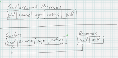
To make the table satisfy 1NF, we need to move the boat information to a new table. In the new table we still are not allowed to store each set of ids in 1 column, and we can’t just add an arbitrary number of columns to the new table (how would we know how many to add?). We instead put each boat id in its own row and also add a foreign key back to the original table so that all the original information is preserved. So this is kind of like a lossless decomposition but we’re fixing a disallowed kind of column instead of a bad functional dependency.

Finally, here are before and after schema diagrams illustrating the decomposition.

Second Normal Form (2NF)

A relation is in second normal form (2NF) if it is in 1NF and does not contain any functional dependencies of the form part of a composite candidate key → non-prime columns.

In practical, I308 terms where we don’t often have candidate keys, this means that if we have a composite primary key, then we can’t have a functional dependency on just part of of that primary key.

Note that 2NF is more restrictive than 1NF because a table can only satisfy the 2NF condition if it also satisfies the 1NF condition. This is typical of the normal forms; they build on each other.

We also have gotten to our first normal form that discusses FDs. Note that it also mentions composite keys. Remember a composite key is one that contains more than one column. The Reservations table above has a PK of sid, bid, date; it has a composite primary key. Tables with a single-column primary key don’t come into play with 2NF. If a table satisfies 1NF and has a single-column primary key, then it automatically satisfies 2NF.

Back to the Reservations table. It does not satisfy 2NF. So far we have seen 0NF (least restrictive), 1NF (more restrictive), and 2NF (most restrictive). The original Reservations table before decomposition satisfies 0NF and 1NF but not 2NF. It does not satisfy 2NF because sid is part of its composite primary key AND there is an FD on sid (sid is the left hand side of an FD; sid comes before the arrow in an FD). Since the most restrictive normal form Reservations satisfies in 1NF we say that “Reservations is 1NF” or “Reservations is in 1NF” or “Reservations satisfies 1NF”.

Because Reservations does not satisfy 2NF, it has a “bad” functional dependency. 2NF tells us exactly how to identify one kind of a bad FD; an FD on part of the primary key is “bad” mkay. If we want Reservations to satisfy 2NF, we have to remove the bad FD. We have to decompose Reservations to eliminate redundancy.

This is how normal forms are used in database design. A data modeler will have some “target” normal form in mind for the database or in mind for each table in the database, and they will examine the FDs to ensure each table meets the target normal form. Any tables that do not meet the target will be de decomposed to eliminate redundancy until the target is met.

The paragraph above mentions to ways of characterizing the target–a single target for the entire database or a target normal form for each table. We’ve already seen what it means for a table to be in a normal form or satisfy it. The normal form a table satisfies is the most restrictive normal form for that table. We can extend this notion an entire database. The normal form of a database is the least restrictive normal form of any table in the database. If we have some tables in a database that are 1NF and some that are 2NF, we say the database satisfies 1NF because every table in the database meets the 1NF conditions. Since not every table meets the more restrictive 2NF, it would not be accurate to claim the entire database does. We err on the side of caution by choosing the least instead of most restrictive among the tables.

Boyce-Codd Normal Form (BCNF)

A relation satisfies Boyce-Codd Normal Form if it is in 2NF and has no functional dependencies on non-prime columns. (In other words, the only allowed FDs are of the form candidate key → other columns)

Now that BCNF has been defined, we can revisit the law we saw above:

Data should depend on the key (1NF), the whole key (2NF), and nothing but the key (BCNF), so help me Codd.

Let’s imagine that we also keep track of dues sailors pay, so we also have a non-prime dues column in the Sailors table. Now here’s the part that violates BCNF: we calculate the dues based on the Sailors rating. Better sailors pay less, perhaps because they bring good publicity to the club. That means that the Sailors table in this case has these FDs: sid → sname, age, rating, dues and rating → dues. rating → dues is “bad” because it violates BCNF since rating is not a key of the table; rating is non-prime. The bad FD causes redundancy because all sailors with a particular rating will also have the same dues value. To fix this bad FD, we decompose this Sailors table to eliminate the redundancy:

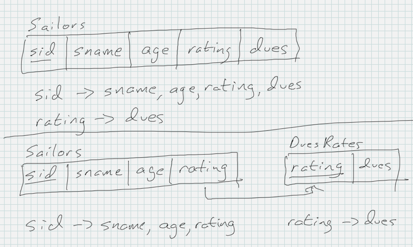
After decomposition, we still have the same two FDs, but they are on different tables now. On the new tables, both are PK → non-prime columns, and all is well. Both tables are BCNF.

Which Normal Form is Right for Me?

Most relational databases ensure their schema is BCNF. You can go far by simply doing this, too. If you are dealing with very specialized situations, you may make other choices. There are actually higher normal forms, and they don’t necessarily simply involve FDs beyond this point. If you need to know more about them, you need to take a graduate-level database course! There’s also one lower normal form we didn’t cover, but it’s optional. The order from least to most strict is 1NF < 2NF < 3NF < BCNF. BCNF is often called “3.5NF” because 3NF and BCNF are so similar. 3NF is older, and BCNF is simpler. Simplicity wins in I308, so we’re ignoring 3NF. If you want to know why, read the optional section below.

Optional Section: Third Normal Form (3NF)

A relation is in third normal form if it satisfies second normal form and it does not have any functional dependencies of the form non-prime column(s) → other non-prime columns

This almost seems like BCNF, because in BCNF we’re not allowed to have FDs on any non-prime columns (nothing but the key!). The difference here is we’re allowed to have FDs of the type some prime column(s) → other prime column(s). What this means in practice is that part of one candidate key may determine part of another. When tables have multiple candidate keys, they are modeling something more complicated than a record with a nice, unique id column. They are likely modeling two inter-related concepts that could be separated into two separate tables. The BCNF wikipedia page gives an example of such a table if you’re curious.