Recap of frequency measures
In a previous topic we defined the cf, df, idf, and tf scores for terms and/or documents in a corpus. Out of these scores each took a term t as its argument, but the term frequency also depended on the document d. In other words, the cf, df, and idf scores measure something only about search terms. The tf score measures something about a term in a particular document. In particular, we can compare tf scores for two different documents using the same term. For instance tf(‘cat’, d1) > tf(‘cat’, d2) means that document d1 is more about ‘cat’ than document d2 is because d1’s tf score for that term is larger–higher tf means a document should score higher for that term.
We also saw that a low df makes for a good search term. The df is inependent of the document–it means some terms should contribute more to a documents score than other because some search terms are more useful. The more useful terms appear in fewer documents, so they can return more specific results. If df(‘cat’) < df(‘dog’), then there are fewer ‘cat’ documents in our corpus, and we should consider ‘cat’ a more useful term than ‘dog’ for ranking our results when they both appear in the same query.
The only problem with df is that we would like to have high scores be better than low scores when we score documents for ranked IR. The easy way to convert a low df (good score) into a numerically larger score is to take it’s reciprocal, 1/df. That idea leads to the idf score. High idf scores are better: idf(‘cat’) > idf(‘dog’) means there are fewer cat documents in our corpus, and we should consider ‘cat’ a more useful term than ‘dog’ for ranking our results when they both appear in the same query.
The tf-idf score
The tf-idf score combines both of these ideas into one score for a term in a document. A high tf-idf score means at least one of these statements is true: 1. the document is very much about that term (high tf score) or 2. the term is a very useful one (relatively few documents in the corpus–high idf score).
Bag of Words Model
The vector space model is an example of a “bag of words” model. In a bag of words model, no effort is made to use the ordering of the words in a document. Instead the document is just treated like it’s a “bag of words”! “Tom is better than Mary”, “Mary is better than Tom”, and “is Mary Tom than better” are all equally good matches to any search term as far as bag of words is concerned. As the example illustrates, bag of words models make no effort to determine if the document make sense. This not necessarily a huge weakness, it’s more that bag of words model are a simple approach and lack the sophistication of models that would attempt to discover the meaning in a document by noting, for instance, that words appear in a certain order or close together in a document.
The term-document incidence matrix
The Vector Space Model (VSM) treats each document in a corpus as a list of numbers, a document vector. Each number in the document vector is a tf-idf score, so there is one entry per term in the document vector. To build up to that concept, we first consider a simpler one. The term-document incidence matrix indicates, for each term in each document, whether or not that term is in the document. The example below from our reading using the plays of Shakespeare as a corpus.
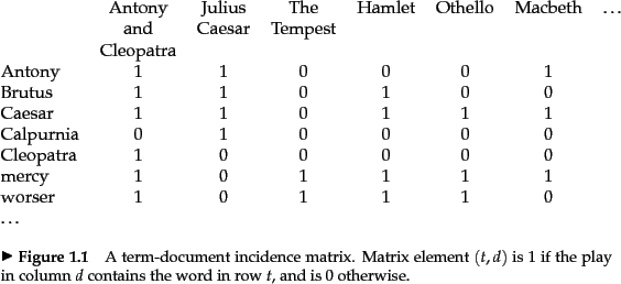
Information equivalent to this matrix is actually computed when we build a frequency index. For every document, we tokenize that document to get its terms. Every term we encounter in a document corresponds to a 1 in the matrix above. We don’t worry about duplicates in this matrix since each entry is either 0 or 1, so it relates to the document frequency which also ignore duplicates. Hopefully you can look at the matrix and convince yourself that adding up each row in the matrix will give you the document frequency for that row’s term.
Term-document count matrix
The next step towards full-blown document vectors is the term-document count matrix where replace each 1 in the matrix above with the term frequency of that term in the document.
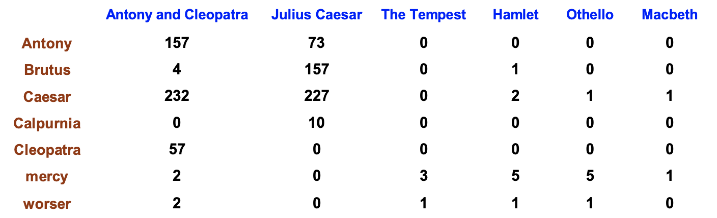
We described the tf score as a way to figure out which document was “most about” a term. The highest tf score in a row is the document most about that term. Hopefully you can also convince yourself that the sum of the numbers in each row gives the collection frequency for that term’s row.
Once again, our frequency index computed this matrix as it scanned the corpus, for it keeps track of the tf score of token it encounters in a document.
Document Vectors
We justified the tf-idf score as including not only the tf score’s contribution described above but also the term’s contribution. Some terms are more important than others, and the most important terms have the highest idf scores! We can incorporate this last piece of information by replacing all the nonzero entries with tf-idf scores to yield the matrix shown below.
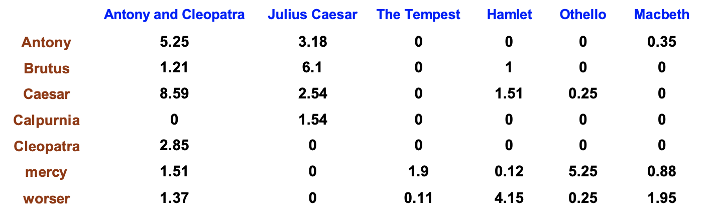
Every document in the corpus in the vector space model is considered to be a vector–a list of numbers where each number is a tf-idf score. The length of each document vector is |V|, the number of words in the vocabulary, and each document’s list is in the same order. We can think of it almost like a dictionary. The first component of the document vector for this corpus is the “Antony” component, the second the “Brutus” one, and so on. Not every document contains all possible search terms, so many entries in the document vector may be 0. This is a feature and not a bug of the vector space model which we’ll get to eventually see!
Document Similarity
Once this correspondence between a document and its lists of tf-idf scores for every term in the vocabulary has been made, it is possible to determine how similar two document are to each other. In this way, one can find the two most similar documents in a corpus, or one can single out a document and rank all the other documents in terms of how similar they are to the chosen document. By the same method, we can rank documents by how similar they are to a query. The best search result in the Vector Space Model is the document that is most similar to the query. The second-best result is the second most similar document, and so on! The cosine similarity is the scoring function that can compute this similarity between the two lists of numbers. It gets its name because it measures the cosine of the angle between two vectors in the vector space model. The cosine function is good for scoring because it varies between 0 and 1 for document vectors. (The full range of cosine is from -1 to 1, but since document vectors have nonnegative components, only the range 0 to 1 is in play corresponding to angles from -90° to +90°.) There are many, many good text search engines that do nothing other than use the Vector Space Model and rank documents based on that. It works that well! We will see how to do that in this two-class topic.
We can think of the cosine similarity score as a function that takes two vectors and returns a single number between 0 and 1 inclusive with 1 indicating the best possible score (the document vectors are as similar as can be) and 0 the worst score (the documents have nothing in common). In more detail, two documents with a cosine similarity score of 1 have the same distribution of all the same terms. They don’t have to be identical because 1) the terms don’t have to be in the same order in this bag of words model and 2) duplication could happen so that “mary had a lamb” and “mary had a lamb mary had a lamb” could have a similarity score of 1. A score of 0 means the two documents don’t have any terms in common except for possibly stopwords we’re ignoring.
In terms of the angle θ between the vectors, two equivalent documents have an angle of 0 between their vectors–the two vectors are parallel to each other. Two completely dissimilar documents would have an angle of either +90° or -90° between them. So the cosine of the angle θ acts to transform small angles (0° ) to high ones (+1) we can use for scoring. Similarly, it transforms high angles ( ±90°) to low scores (0).
We can compute the cosine similarity score for every pair of documents in the corpus, and the highest-scoring pair is the two most similar documents. By sorting the scores, we can sort the pairs based on similarity. This approach is used often in recommender systems in order to determine or recommend to the user documents that are more similar to the one they’re currently viewing.
We’ll also see that queries can be turned into vectors, too, and that means we can compute how similar every document is to the query. The most similar document to the query will have the highest cosine similarity with the query, and it will be the best search result according to the VSM. The second highest scoring document is the second best result, and so on. This scoring against a query vector is the main way we’ll use the VSM in I417.
To compute any of these scores, we must find the cosine of the angle between two vectors, and we use a function called the dot product or scalar product for that calculation.
Dot products
The cosine similarity score is based on the dot product between two vectors. Another name for the dot product is the scalar product–they both mean the same thing. The dot product or scalar product is a mathematical operation that takes two vectors and returns a single number. We can think of it like a function because it takes two arguments–two lists of numbers–and gives us a single number as its return value. In fact, we wrote this very function earlier in the semester on a homework assignment! Here is the code from the solution to that assignment:
def dot_product(v1, v2):
    dot_prod = 0
    for i in range(len(v1)):
        dot_prod += v1[i]*v2[i]

    return dot_prod
The formula implemented in that code indicates we can multiply two vectors of the same length component by component and add up the sum of those products to get the dot product. That’s it! If you think about a vector as a list of numbers like [1,2,3]. The first component is 1, the second 2, and so on. For two vectors like [1, 2, 3] and [10, 20, 30], the dot product is 1*10 + 2*20 + 3*30 = 140. We’re not stuck using only 3-dimensional vectors, though. The dot product works for any number of entries, and so does our function.
There’s one other way to write the dot product that uses a different formula based on the magnitude of each vector. Lo and behold, we also wrote a function for that because the magnitude is the square root of the sum of the squares of the components of a vector:
def vector_magnitude(v):
    v_mag = 0
    for val in v:
        v_mag += val**2
    v_mag = v_mag**0.5

    return v_mag
The magnitude of a vector v is usually written like |v|, and dot product of two vectors u and v is usually written as u⋅v. That dot in between them why it’s often called the dot product, as a matter of fact. It’s called the scalar product because a scalar is a single number in contrast to the multiple numbers in a vector, and the dot product of two vectors is a scalar and not another vector. Now we can get to the other formula for the dot product.
u⋅v = |u| |v| cos θ
The neat thing about this formula is that it uses information from geometry. If you measure the length (magnitude) of each vector with a rule and the angle between them with a protractor, you can calculate the dot product.
Cosine Similarity Score Formula
In our case, though, we can’t use rulers and protractors, and we wouldn’t know what an angle between two document vectors that are 10,000 numbers long might mean. What we do know are those numbers–the components of the vectors because each is a tf-idf score we calculated when we built the index. Since we know the components of the two vectors, then we can calculate the length or magnitude of each vector with one of our functions or formulas and we can calculate the dot product with the other one. The only thing we don’t know from the formula is the cosine of the angle between them, so we can solve for that. That gives us the cosine similarity formula for two vectors
cos θ = u⋅v / (|u| |v|)
The cosine similarity can only vary between 0 and 1, and it’s only equal to 1 when the vectors are parallel to each other. That’s what makes it a useful score–two similar documents will have similar proportions of tf-idf scores for each term in the document, and the cosine similarity score can equate that with a number.
We can turn that formula above into code using the functions we already have:
def cos_similarity(v1, v2):
    v1_mag = vector_magnitude(v1)
    v2_mag = vector_magnitude(v2)
    v1dotv2 = dot_product(v1, v2)

    # check for divide by zero in real life

    return v1dotv2/(v1_mag * v2_mag)
A nifty way to optimize our thinking about this is to recognize that
|u|² = u⋅u
That lets us just use the dot_product() function to calculate the cosine similarity:
def cos_similarity(v1, v2):
    v1_mag_squared = dot_product(v1, v1)
    v2_mag_squared = dot_product(v2, v2)
    v1dotv2 = dot_product(v1, v2)

    # check for divide by zero in real life

    return v1dotv2/math.sqrt(v1_mag_squared * v2_mag_squared)
The Query Vector
The key idea that makes the VSM work for Ranked IR is that a query on a corpus can be thought of as a vector, too! Since documents are vectors in the VSM and queries are, too, that suggests that we can thinking of each query as a document in the corpus. The documents must similar to that query document must be the the best results for that query. That’s the essence of the Vector Space Model!
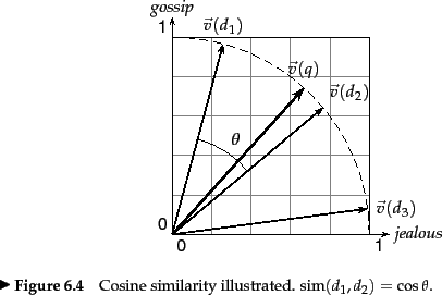
Making the query vector is simple in the VSM. We imagine all its entries being 0 except for the actual query terms which we imagine having 1’s for entries. In the example below from The IR Book, for a two-word vocabulary where a vector has “jealous” and “gossip” components, the query vector would be [1,1]. In 2D this vector will lie along the line y = x at 45° to the horizontal (x) axis, and that fact makes it easy to spot the query vector in figures such as this.
In this two-word vocabulary, we can enumerate all the possible queries. The query “jealous” will have the vector [1,0] while the query “gossip” has the vector [0,1]. We’ve already seen that “jealous gossip” or “gossip jealous” have the vector [1,1]. For any of these query vectors, we compute the cosine similarity score of the query vector with all documents in the corpus and sort the documents from high score to low score.
Implementing the cosine similarity in Ranked IR
The final thing to think about with the vector space is what the query vector looks like for a typical corpus with a large vocabulary. To be specific, let’s imagine the vocabulary is 100,000 words so that each document vector and the query vector is in general a list of 100,000 numbers. In the document vector, the 100,000 numbers are tfidf scores for each term in that document. We can think of each component as being labeled by the term, so instead of x, y, … components or 0, 1, 2, components we can still think of the “gossip” component, the “jealous” component, the “cat” component, the “dog” component, and so on. Not every document contains every term, so there are typically many entries in the document vector that are 0. A vector or other large numerical data structure with many 0 entries and relatively few nonzero ones is said to be sparse. Document vectors are sparse.
Query vectors are even more sparse! If we have the same “gossip jealous” query on our corpus with a 100,000 word vocabulary, then the the query vector will have 2 nonzero entries because the “gossip” and “jealous” components will both be 1 but the other 999,998 components will be 0’s.
The dot product is the numerator in the cosine similarity score, and that dot product between a document vector D and the query vector Q will look like
D⋅Q = D[‘gossip’]*Q[‘gossip’] + D[‘jealous’]*Q[‘jealous’] + D[‘cat’]*Q[‘cat’] + D[‘dog’]*Q[‘dog’] + …
From what we’ve seen about the query vector, the only two nonzero terms are the first two. All the other terms in the sum don’t matter! So we can effectively ignore the nonzero terms since they won’t contribute to the numerator.
D⋅Q = D[‘gossip’]*Q[‘gossip’] + D[‘jealous’]*Q[‘jealous’] # all other terms are 0!
Moreover, the two entries that are nonzero are 1, so we can even leave them out of the multiplication.
D⋅Q = D[‘gossip’] + D[‘jealous’] # using only the terms where the Q component is 1
At this point, we have gotten to an important optimization for the vector space model. Once we have the query and the documents in the result set, we can compute the dot product between a document vector and the query vector simply by summing each document vector’s components that are in the query. Since each component is a tfidf score, we’re adding up tfidf scores for the query term in each document. That’s not the entirety of the cosine similarity, but it’s the numerator. Now we just need to work on the denominator.